Supported grid formats
pyshtools makes use of grid formats that accommodate exact quadrature. These include regularly spaced grids that satisfy the Driscoll and Healy (1994) sampling theorem, and grids for exact quadrature using Gauss-Legendre quadrature [e.g., Press et al. 1992]. The grids are input as arrays where the rows and columns correspond to equal values of latitude and longitude, respectively. The first row corresponds to the latitude band closest to the north pole, and the first column corresponds to 0 degrees E.
Gauss-Legendre Quadrature
For the case of Gauss-Legendre quadrature (GLQ), the quadrature is exact when the function \(f\) is sampled in latitude at the \((L+1)\) zeros of the Legendre Polynomial of degree \((L+1)\). Since the function also needs to be sampled on \((2L+1)\) equally space grid nodes for the Fourier transforms in longitude, the function \(f\) is sampled on a grid of size \((L+1)\times(2L+1)\). The redundant data points at 360\(^{\circ}\) E longitude are not required by the spherical harmonic transformation routines, but can be computed by specifying the optional argument extend.
Driscoll and Healy [1994]
The second type of grid is for data that are sampled on regular grids. As shown by Driscoll and Healy [1994], an exact quadrature exists when the function \(f\) is sampled at \(N\) equally spaced nodes in latitude and \(N\) equally spaced nodes in longitude. For this sampling (DH), the grids make use of the longitude band at 90\(^{\circ}\) N, but not 90\(^{\circ}\) S, and the number of samples is \(2(L+1)\), which is always even. Given that the sampling in latitude was imposed a priori, these grids contain almost twice as many samples in latitude as the grids used with Gauss-Legendre quadrature. It should be noted that for this quadrature, the longitude band at 90\(^{\circ}\) N is ultimately downweighted to zero, and hence has no influence on the returned spherical harmonic coefficients.
For geographic data, it is common to work with grids that are equally spaced in degrees latitude and longitude. pyshtools provides the option of using grids of size \(N\times2N\), and when performing the Fourier transforms for this case (DH2), the coefficients \(c_{lm}\) and \(s_{lm}\) with \(m>L\) are discarded. The redundant data points at 360\(^{\circ}\) E longitude and the latitudinal band at 90\(^{\circ}\) S are not required by the spherical harmonic transformation routines, but can be computed by specifying the optional argument extend.
Comparison of DH and GLQ grids
The properties of the Driscoll and Healy [1994] and Gauss-Legendre Quadrature grids are summarized in the following table:
| DH1 | DH2 | GLQ | |
|---|---|---|---|
| Name | Driscoll and Healy | Driscoll and Healy | Gauss-Legendre Quadrature |
| Shape (\(N_{lat} \times N_{lon}\)) | \(N \times N\) | \(N \times 2N\) | \(N \times 2N\) |
| \(L\) | \(N/2-1\) | \(N/2-1\) | \(N-1\) |
| \(N\) | \(2L+2\) | \(2L+2\) | \(L+1\) |
| \(\Delta \theta\) | \(180^{\circ}/N\) | \(180^{\circ}/N\) | Variable |
| \(\Delta \phi\) | \(360^{\circ}/N\) | \(180^{\circ}/N\) | \(360^{\circ}/(2N-1)\) |
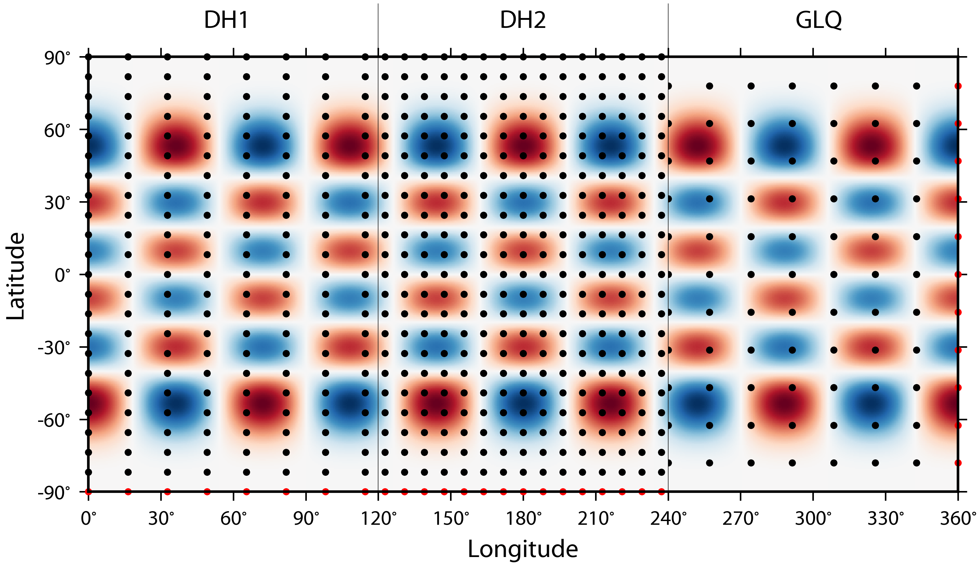
The figure below demonstrates how these grids sample an arbitrary function that has a maximum spherical harmonic degree of 10. The DH1 and DH2 grids are seen to have the same sampling in latitude, but the DH2 grid has twice as many samples in longitude than does the DH1 grid. The GLQ grid is regularly sampled in longitude, but is irregularly sampled in latitude. Given the freedom associated with choosing the latitude coordinates for the GLQ grids, these grids have about half as many latitudinal points as do the more regular DH grids. The red points at the south pole and 360\(^{\circ}\) E are not required when performing the spherical harmonic transforms, but can be computed by specifying the optional argument extend.
References
-
Driscoll, J. R. and D. M. Healy, Computing Fourier transforms and convolutions on the 2-sphere, Adv. Appl. Math., 15, 202-250, doi:10.1006/aama.1994.1008, 1994.
-
Press, W. H., S. A. Teukolsky, W. T. Vetterling, and B. P. Flannery, “Numerical Recipes in FORTRAN: The Art of Scientific Computing,” 2nd ed., Cambridge Univ. Press, Cambridge, UK, 1992.