Numerical computations
Spherical harmonic reconstructions
If the spherical harmonic coefficients of a function \(f\) were known up to a maximum degree \(L\), the function could be evaluated at arbitrary colatitude \(\theta\) and longitude \(\phi\) using the equation
\begin{equation} f\left(\theta,\phi\right) = \sum_{l=0}^{L} \sum_{m=-l}^l f_{lm} \, Y_{lm}\left(\theta,\phi \right). \end{equation}
Using the separate variables \(C_{lm}\) and \(S_{lm}\) for the cosine and sine spherical harmonic coefficients, respectively, and after interchanging the order of summations over \(l\) and \(m\), the function can be expressed equivalently as
\[\begin{equation} f\left(\theta,\phi\right) = \sum_{m=0}^L \sum_{l=m}^{L} \left( C_{lm} \, \bar{P}_{lm}(\cos \theta) \, \cos m\phi + S_{lm} \, \bar{P}_{lm}(\cos \theta) \, \sin m\phi\right). \end{equation}\]Defining the two component vector
\[\begin{equation} \left[a_m(\theta), b_m(\theta)\right] = \sum_{l=m}^{L} \left[C_{lm}, S_{lm}\right] \, \bar{P}_{lm}(\cos \theta), \end{equation}\]The function \(f\) can be written more simply as
\[\begin{equation} f\left(\theta,\phi\right) = \sum_{m=0}^L \left( a_m(\theta) \, \cos m\phi + b_m(\theta) \, \sin m\phi\right). \end{equation}\]For a given latitude band, the function \(f\) can thus be evaluated on a series of grid nodes all at the same time using an inverse fast Fourier transform. For this operation, SHTOOLS makes use of the highly optimized software package FFTW [Frigo and Johnson 2005] that supports grids of arbitrary length and both real and complex data. To adequately sample the function in longitude, a minimum of \(2L+1\) data points should be employed.
The coefficients \(a_m\) and \(b_m\) depend upon the associated Legendre functions, which are calculated efficiently using standard three-term recursion relations over adjacent spherical harmonic degrees. For a given colatitude, the sectoral term \(\bar{P}_{mm}\) is first calculated using an analytic equation, and then \(\bar{P}_{lm}\) is calculated for all values of \(l>m\). To circumvent numerical underflows near the poles for large values of \(m\), the associated Legendre functions are calculated using the approach of Holmes and Featherstone [2002], where the sectoral \(\bar{P}_{mm}\) terms are multiplied by \(10^{280} \sin^m \theta\) prior to performing the recursions, and then appropriately unscaled at the end of the recursion. This ensures that the Legendre functions are accurate to about degree 2800.
Spherical harmonic transforms
The spherical harmonic coefficients of a function can be calculated from the relation
\[\begin{equation} \left[C_{lm}, S_{lm}\right] = \frac{1}{4\pi} \int_{0}^{2\pi} \int_0^{\pi} f(\theta,\phi) \, \bar{P}_{lm}(\theta) \left[\cos m\phi, \sin m\phi\right]\, \sin\theta \, d\theta \, d\phi. \end{equation}\]Defining the two intermediary variables \(c\) and \(s\)
\[\begin{equation} \left[c_{lm}^{(i)}, s_{lm}^{(i)}\right] = \int_0^{2\pi} f(\theta_i,\phi) \left[ \cos m\phi, \sin m\phi\right] d\phi, \end{equation}\]it is seen that for a given colatitude \(\theta_i\) and degree \(l\), all of the angular orders can be calculated at once by making use of a fast Fourier transform of the function \(f\). Replacing the integral over latitude with a numerical quadrature rule, the spherical harmonic coefficients can be calculated as
\[\begin{equation} \left[C_{lm}, S_{lm}\right] = \frac{1}{4 \pi} \sum_{i=1}^N w_i \, \bar{P}_{lm}(\cos \theta_i) \left[c_{lm}^{(i)}, s_{lm}^{(i)}\right]. \label{eq:quadrature} \end{equation}\]Here, \(w\) is the latitudinal weight, and \(N\) is the number of latitudinal points over which the integration is performed. It is possible to choose the weights \(w_i\) and the locations of the latitudinal sampling points \(\theta_i\) such that the quadrature in equation \eqref{eq:quadrature} is exact.
As is described in more detail here, SHTOOLS makes use of grid formats that accommodate exact quadrature.These include regularly spaced and sampled grids that satisfy the Driscoll and Healy (1994) sampling theorem, and grids for exact quadrature using Gauss-Legendre quadrature [e.g., Press et al. 1992]. For all grids, the quadrature is exact only when the function being integrated is a terminating polynomial. The functions \(c_{lm}\) and \(s_{lm}\) can be approximated as polynomials of maximum degree \(L\), and when multiplied by the associated Legendre function, the integrand is approximately a polynomial of maximum degree \(2L.\)
Accuracy
To test the accuracy of the spherical harmonic transforms and reconstructions, two sets of synthetic spherical harmonic coefficients were created. Each coefficient was chosen to be a random Gaussian distributed number with unit variance, and the coefficients were then scaled such that the power spectrum was proportional to either \(l^2\) or \(l^{-2}\). For a given spherical harmonic bandwidth \(L\), the function was reconstructed in the space domain using the Gauss-Legendre quadrature implementation and then re-expanded into spherical harmonics. The maximum and root-mean square (rms) relative errors between the initial and final set of coefficients were then computed as a function of spherical harmonic degree, as plotted in the figure below.
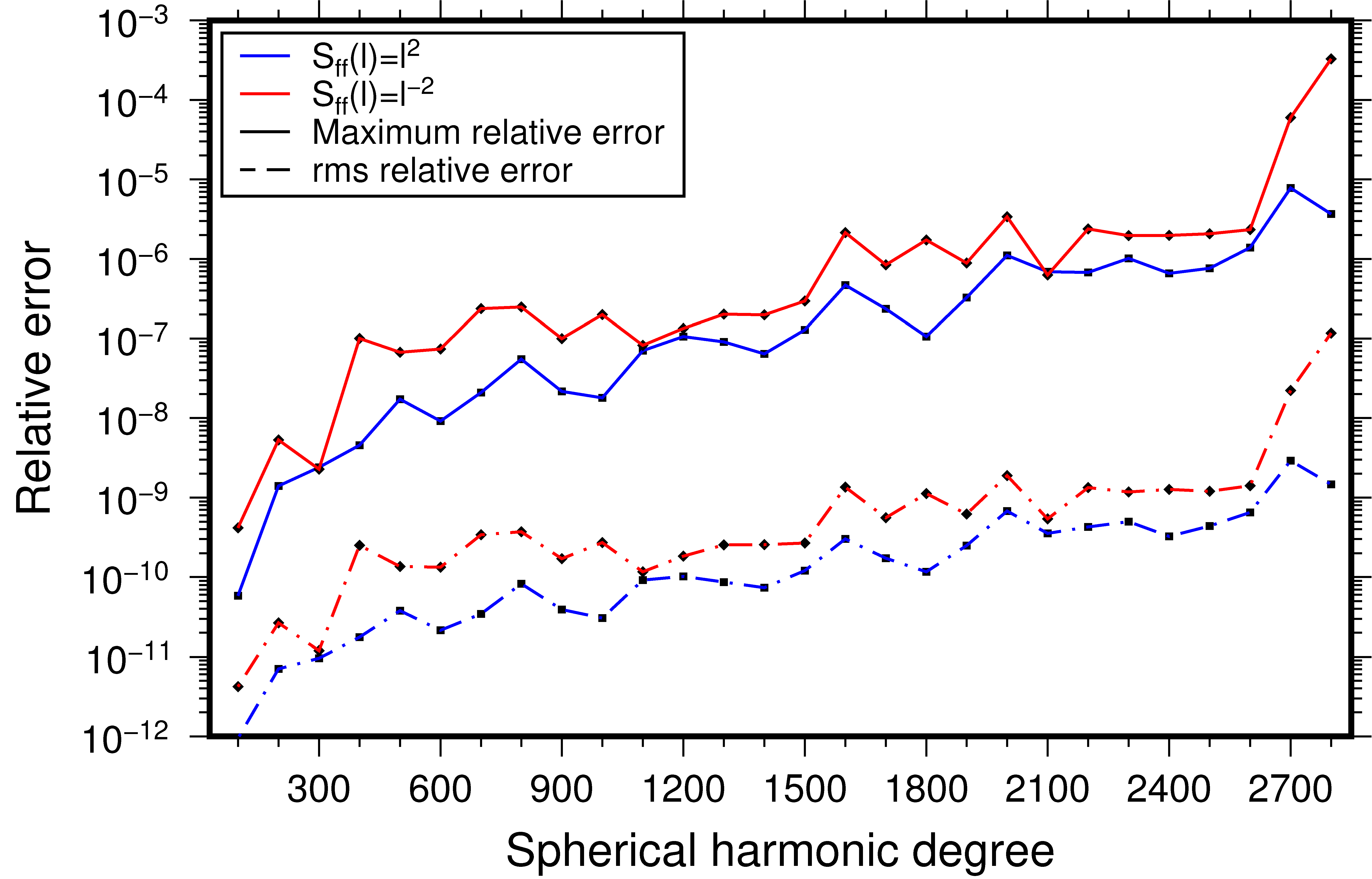
The errors associated with the transform and inverse pair increase in an quasi-exponential manner, with the maximum relative error being approximately 1 part in a billion for degrees close to 400, and about 1 part in a million for degrees close to 2600. Though the errors are negligible to about degree 2600, they then grow somewhat between degrees 2700 and 2800. The rms errors for the coefficients as a function of the bandwidth \(L\) are typically three orders of magnitude smaller than the maximum relative errors.
The relative errors are nearly the same for the two tested power spectra, implying that the form of the data do not strongly affect the accuracy of the routines. Relative errors using the Driscoll and Healy [1994] sampled grids are nearly identical to those using Gauss-Legendre quadrature. The errors associated with the routines for complex data are lower by a few orders of magnitude.
Timing tests
The speed of the spherical harmonic reconstructions and transforms were tested for both real and complex data using the Gauss-Legendre and Driscoll and Healy [1994] quadrature implementations. The amount of time in seconds required to perform these operations is plotted in the figure below as a function of the spherical harmonic bandwidth of the function. These calculations were performed on a modern Mac Pro 2.7 GHz 12-Core Intel Xeon E5 using 64 bit executables and level 3 optimizations.
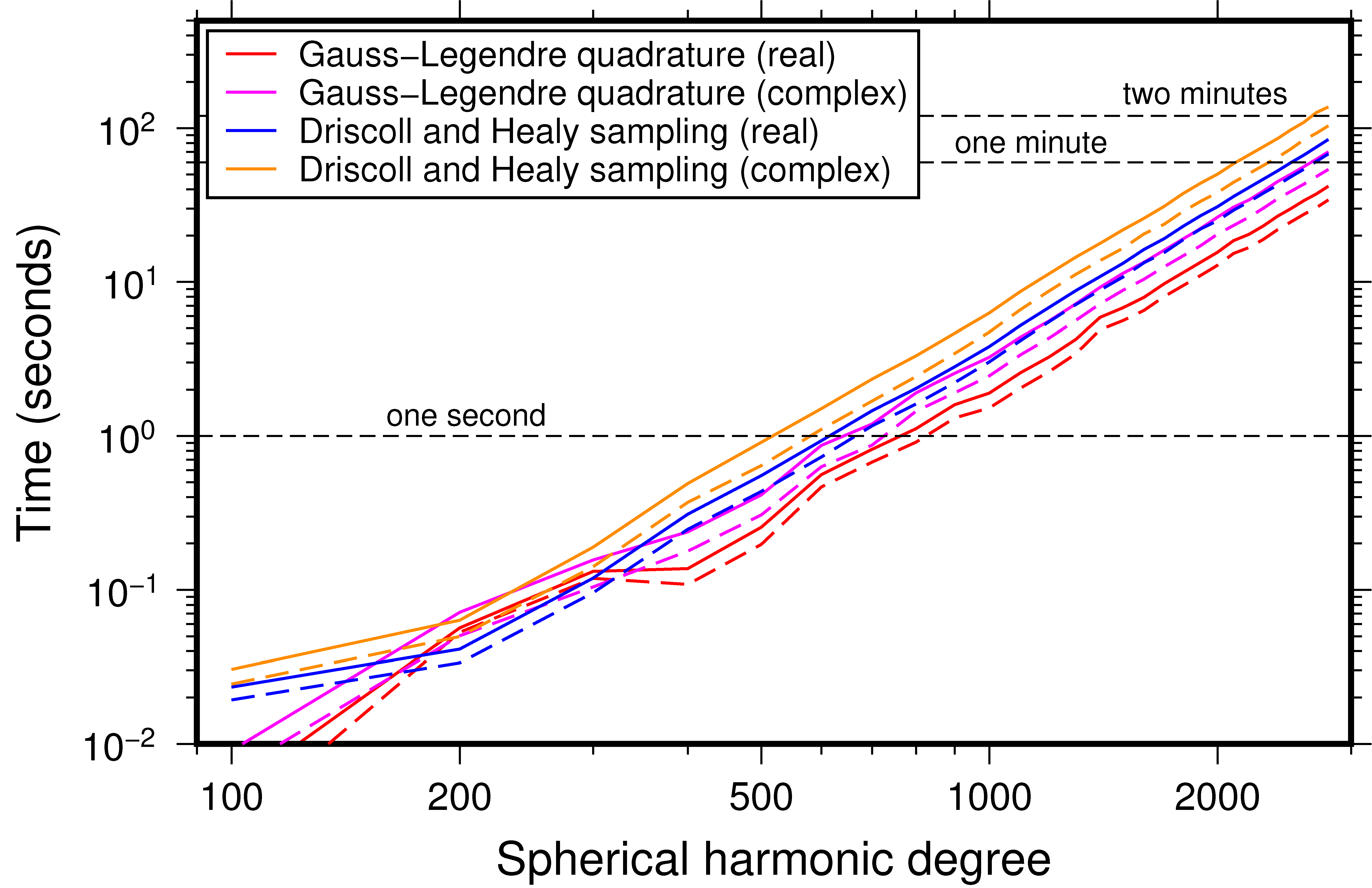
For the real Gauss-Legendre quadrature routines, the transform time is on the order of one second for degrees close to 800 and about 30 seconds for degree 2600. For the real Driscoll and Healy [1994] sampled grids, the transform time is close to a second for degree 600 and about 1 minute for degrees close to 2600. The complex routines are slower by a factor of about 1.4.
References
-
Driscoll, J. R. and D. M. Healy, Computing Fourier transforms and convolutions on the 2-sphere, Adv. Appl. Math., 15, 202-250, doi:10.1006/aama.1994.1008, 1994.
-
Frigo, M., and S. G. Johnson, The design and implementation of FFTW3, Proc. IEEE, 93, 216-231, doi:10.1109/JPROC.2004.840301, 2005.
-
Holmes, S. A., and W. E. Featherstone, A unified approach to the Clenshaw summation and the recursive computation of very high degree and order normalised associated Legendre functions, J. Geodesy, 76, 279-299, doi:10.1007/s00190-002-0216-2, 2002.
-
Press, W. H., S. A. Teukolsky, W. T. Vetterling, and B. P. Flannery, “Numerical Recipes in FORTRAN: The Art of Scientific Computing,” 2nd ed., Cambridge Univ. Press, Cambridge, UK, 1992.